Drawing the Four Neural Networks that Changed AI
Making beautiful visualizations and writing about AI’s most influential models with PlotNeuralNet

I’ve recently been writing a paper where we developed a new model architecture and I wanted a nice way of representing it in a figure. My first instinct was to jump into Adobe Illustrator. I fiddled around with the vertices of my fourth cube feebly trying to get the perspective right. That’s when it hit me: “I’m a programmer. Surely, there’s a tool out there for this.”
After scouring countless Github repositories, I stumbled upon a real gem that made my earlier attempts look like child’s play. It got me inspired to generate diagrams of some of history’s most influential neural networks and write a bit about them and their authors in this article.
If you too want to create your own diagrams of these architectures, I’ll also show you how to use the PlotNeuralNet package to generate them.
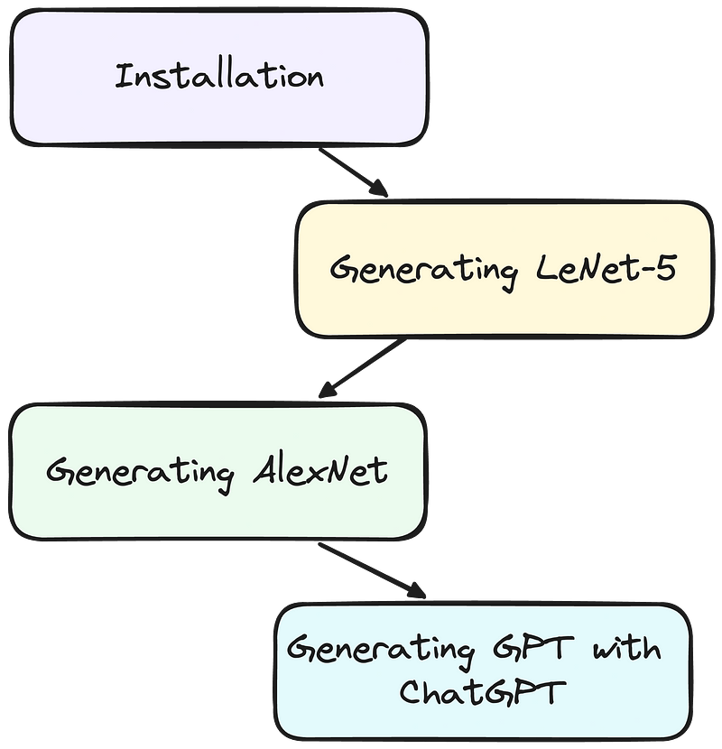
This article is broken up into the following four parts. Feel free to jump around to a section relevant to you. If you just want to read about a history of neural networks, then skip the installation step, and start reading!
- Installation
- Generating LeNet-5 — the network that showed deep learning could beat out traditional machine learning to recognize numbers
- Generating AlexNet — the network that brought deep learning to the forefront of image classification
- Generating GPT with ChatGPT — generating the network that made deep NLP usable for the masses with itself
Installation
If you want to follow along and draw these diagrams yourself, start by installing LaTeX. It’s a really popular markup language for writing. It’s used by a lot of authors, especially those in engineering and computer science for it’s ability to easily create nicely formatted publisher-ready content.
On Mac, if you have homebrew, you can install LaTeX with the MacTeX package with the following command:
brew install --cask mactexOn Linux, you can run the following commands:
sudo apt-get install texlive-latex-base
sudo apt-get install texlive-fonts-recommended
sudo apt-get install texlive-fonts-extra
sudo apt-get install texlive-latex-extra
On Windows, you can:
Download and install MikTeX.
Then on all platforms clone the package:
git clone https://github.com/HarisIqbal88/PlotNeuralNet.gitand change directory to the PlotNeuralNet/Examples/directory. This is where you’ll also save all your files. Running LaTeX code from here will allow LaTeX to find the correct files from PlotNeuralNet to generate your images.
Generating LeNet-5
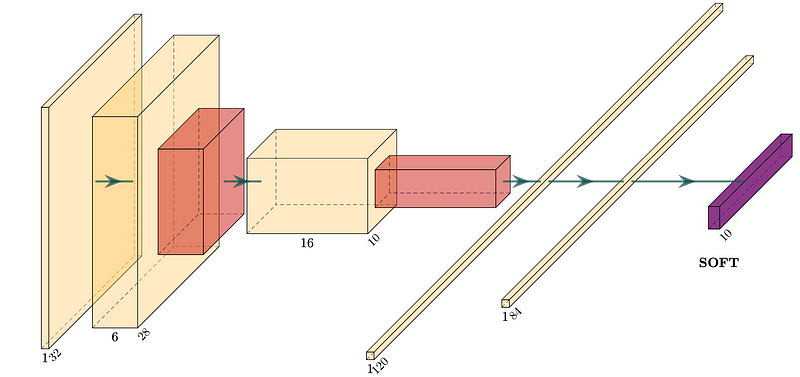
LeNet-5 was the first convolutional neural network. It was created by Yann LeCun and Yoshio Bengio in 1998. They were inspired by earlier work in one of the first neural networks, the Neocognitron, which was created by a 1970s Japanese engineer, Kunihiko Fukushima.
However, LeCun and Bengio made several improvements that brought about the success of their algorithm:
- They had superior training data (the handwritten MNIST digits database)
- Faster processing power, and
- Critically, the backpropogation algorithm, the main algorithm that facilitates learning in neural networks. It allows minimising error for each artificial neuron parameter from error in the output. This process starts all the way at the end/output of the model, going back each of its layers to the start.
This model was one of the first to become sufficiently reliable and an early commercial application of deep learning. It was widely used by the US postal service to automate reading ZIP codes on mail envelopes.

Yann LeCun went on to become the founding director of the New York University Center for Data Science as well as the director of AI research at Facebook. Yoshua Bengio is now a professor at the University of Montreal and co-directs the renowned Machines and Brains program at the Canadian Institute for Advanced Research.
To draw their network, we can create the following TeX file, which we’ll call lenet5.tex
and then run the following command to turn the latex document into a pdf:
pdflatex ./lenet5.texYou should then see a lenet5.pdf file with the diagram from the start of this section.
Generating AlexNet
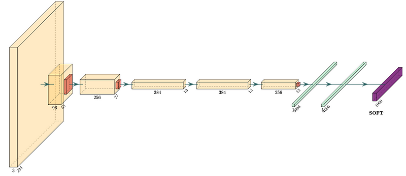
Before this model, Fei-Fei Li created one of the first large image classification datasets, ImageNet. This spawned image classification challenges like the ILSVRC to spur on development in the field.
The first two years of ILSVRC (2010–2011) were dominated by feature-engineering-driven traditional machine learning ideology. In the third year (2012), all entrants except one were traditional machine learning algorithms.
AlexNet was the first entrant using neural networks. It was created by Alex Krizhevsky and Ilya Sutskever working out of a University of Toronto Lab led by Geoffrey Hinton. They absolutely crushed all existing benchmarks with their submission, reducing classification error by 40%. In an instant, deep learning architectures emerged from the fringes of machine learning to the fore.
Their breakthroughs were:
- They had ImageNet, a dataset with millions of images.
- They figured out how to program two GPUs to train their model with previously unseen efficiency,
- They made their architecture far deeper than LeNet and
- They used the Rectified Linear Unit (the activation function of a new type of artificial neuron that is now the most popular neuron used in neural networks) and Dropout (a trick to generalize deep learning models beyond the data they are trained on).
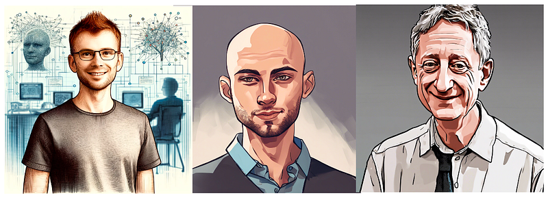
Krizhevsky and Sutskever sold their startup, DNN Research Inc., to Google, shortly after winning the contest. Sutskever went on to be a co-founder and chief scientist at OpenAI. As for Geoffrey Hinton, he is now widely known as “the godfather of deep learning”. He is also an engineering fellow at Google, and was responsible for managing Google’s Brain Team.
To draw their network, we can create the following TeX file, we’ll call alexnet.tex
and then run the following command to turn the latex document into a pdf:
pdflatex ./alexnet.texYou should then see a alexnet.pdf file with the diagram from the start of this section.
Generating GPT with ChatGPT
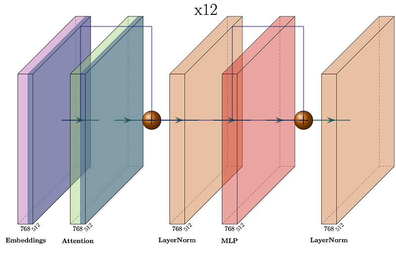
The GPT was one of the first of OpenAI’s large language models following Google’s invention of the transformer architecture in 2017. In 2018, researchers at OpenAI, Alec Radford, Karthik Narasimhan, Tim Salimans and again, Ilya Sutskever, published the first GPT model in their paper, “Improving Language Understanding by Generative Pre-Training”. GPT stands for generative pre-trained transformer and is the first example of the concept.
What makes GPT differ from prior natural language processing (NLP) approaches was its “semi-supervised” approach. It involved an unsupervised generative “pre-training” stage in which a language modeling objective was used to set initial parameters and a supervised discriminative “fine-tuning” stage in which these parameters were adapted to a target task. Additionally, the transformer architecture differed from prior recurrent neural network NLP approaches providing the GPT model with a more structured memory, resulting in a robust transfer performance across diverse tasks.

If you haven’t been living under a rock lately, you’ve seen this architecture in ChatGPT, now using the 3rd and 4th iteration of this model (GPT-3 and GPT-4). These architectures are now a well-kept secret over at OpenAI; however, because the original architecture was publicly released and published, we can draw it below.
For a bit of fun, we’ll see how you can take a printout of the GPT model running in pytorch code, and pass it to a GPT model powering ChatGPT, to then generate our TeX file. You can also do the same with another representation of your model.
Let’s assume you have the following pytorch code, printing your model architecture.
from transformers import OpenAIGPTTokenizer, OpenAIGPTModel
import torch

tokenizer = OpenAIGPTTokenizer.from_pretrained("openai-gpt")
model = OpenAIGPTModel.from_pretrained("openai-gpt")

inputs = tokenizer("Hello, my dog is cute", return_tensors="pt")
outputs = model(**inputs)

last_hidden_states = outputs.last_hidden_state

# now print architecture
print(model)
Now, prompt ChatGPT, or another LLM, with your architecture printout:
Can you generate PlotNeuralNet latex code to generate this GPT architecture?

OpenAIGPTModel(
  (tokens_embed): Embedding(40478, 768)
  (positions_embed): Embedding(512, 768)
  (drop): Dropout(p=0.1, inplace=False)
  (h): ModuleList(
    (0-11): 12 x Block(
      (attn): Attention(
        (c_attn): Conv1D()
        (c_proj): Conv1D()
        (attn_dropout): Dropout(p=0.1, inplace=False)
        (resid_dropout): Dropout(p=0.1, inplace=False)
      )
      (ln_1): LayerNorm((768,), eps=1e-05, elementwise_affine=True)
      (mlp): MLP(
        (c_fc): Conv1D()
        (c_proj): Conv1D()
        (act): NewGELUActivation()
        (dropout): Dropout(p=0.1, inplace=False)
      )
      (ln_2): LayerNorm((768,), eps=1e-05, elementwise_affine=True)
    )
  )
)
and you should receive something similar to the following:
Run the following command to turn the latex document into a pdf:
pdflatex ./gpt.texYou should then see a gpt.pdf file with the diagram from the start of this section.
Each of these architectures brought a unique set of innovations that have brought AI to what it is today. These diagrams are an illustration of the “brains” of these amazing models. To me, it is kind of like taking a walk through an art gallery, where each masterpiece has transformed the landscape of artificial intelligence in its own unique way.
Thanks for taking this stroll with me through a bunch of amazing neural network architectures. Hopefully, it’s sparked your interest to dive deeper, explore more, and maybe even contribute to the next chapter of this exciting field. It may also just help you draw a neural network you’ve been struggling to illustrate. Who knows what the next masterpiece might look like? But one thing’s for sure — it’s going to be a game-changer.


